Hardy, Weinberg Equilibrium: Allele Frequencies, p²+2pq+q², and the χ² Test

Hardy, Weinberg says that in a population that isn’t evolving, genotype frequencies follow p² + 2pq + q² = 1 from the allele frequencies p and q. Get p and q from the genotype counts (p = (2·AA + Aa) / 2N), work out the expected counts, and a chi-square test tells you whether the population is at equilibrium. Do all of it, allele frequencies, expected counts and the χ² verdict, with the Hardy, Weinberg calculator; here’s the reasoning.

The idea in one picture

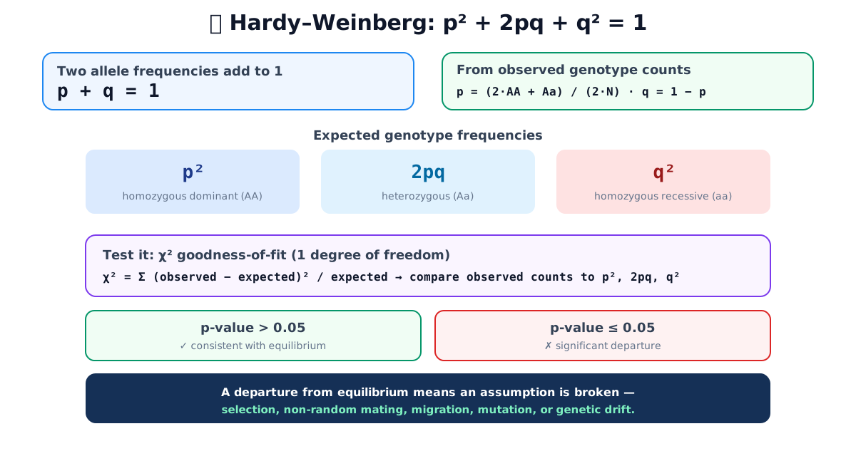
Step 1, allele frequencies from genotype counts

Count the three genotypes and turn them into allele frequencies. Each homozygote carries two copies of its allele, each heterozygote one of each:

p = (2·AA + Aa) / (2N) and q = 1 − p

where N is the total number of individuals. For a classic textbook sample of 298 AA, 489 Aa and 213 aa (N = 1000): p = (2×298 + 489) / 2000 = 1085 / 2000 = 0.5425, so q = 0.4575.

Step 2, expected genotype frequencies

If the population is at equilibrium, the genotype frequencies come straight from p and q:

• p², homozygous dominant (AA)
• 2pq, heterozygous (Aa)
• q², homozygous recessive (aa)

These sum to 1 because (p + q)² = p² + 2pq + q² = 1. Multiply each frequency by N to get expected counts. With p = 0.5425 and q = 0.4575:

• p²·N = 0.5425² × 1000 ≈ 294.3 homozygous dominant
• 2pq·N = 2 × 0.5425 × 0.4575 × 1000 ≈ 496.4 heterozygous
• q²·N = 0.4575² × 1000 ≈ 209.3 homozygous recessive

Notice the expected counts add back to 1000, a quick sanity check that you haven’t dropped a term.

Step 3, test with chi-square

Now compare what you observed to what’s expected under Hardy, Weinberg with a chi-square goodness-of-fit test:

χ² = Σ (observed − expected)² / expected

with 1 degree of freedom (three genotype classes, minus one for the fixed total, minus one for the allele frequency estimated from the data). Working the sum term by term makes the test concrete:

Genotype	Observed	Expected	(O − E)² / E
AA (homozygous dominant)	298	294.3	0.047
Aa (heterozygous)	489	496.4	0.110
aa (homozygous recessive)	213	209.3	0.065
Total	1000	1000	χ² ≈ 0.22

A χ² of about 0.22 on 1 degree of freedom corresponds to a p-value near 0.64, far above 0.05, so the population is consistent with Hardy, Weinberg equilibrium. The comparison point is the χ² critical value for 1 df at the 5 % level, which is 3.841: any χ² below that keeps you in “no significant departure” territory, and a value above it (p ≤ 0.05) signals a significant departure. Here 0.22 is nowhere near 3.841. The Hardy, Weinberg calculator runs this test and gives the plain-English verdict.

Frequencies versus counts, don’t mix them

The single most common error is testing on frequencies instead of counts. The χ² statistic depends on sample size: 30 % versus 33 % is trivial in a sample of 30 and overwhelming in a sample of 30,000. Always feed the test whole-number expected and observed counts (frequency × N), never proportions. The same logic explains why a locus can look off yet pass the test in a small sample, and why huge samples flag departures that are biologically tiny, a large N gives the test the power to notice small deviations.

What a departure means

Hardy, Weinberg is a null model: it describes a population where nothing is changing the allele frequencies. So when observed genotypes depart significantly from the expectation, it means one of the model’s assumptions is being violated:

• Natural selection, some genotypes survive or reproduce better.
• Non-random mating, for example inbreeding, which raises homozygotes.
• Migration (gene flow), alleles entering or leaving the population.
• Mutation, new alleles appearing.
• Genetic drift, random change in a small population.

The test doesn’t tell you which. It tells you that the simple no-evolution model doesn’t fit, which is the starting point for asking why. Each assumption maps to one force it rules out:

Assumption	Force it excludes	What breaks it
No selection	Natural selection	Some genotypes survive or reproduce better
Random mating	Non-random mating	Inbreeding, assortative mating (raises homozygotes)
No migration	Gene flow	Alleles entering or leaving the population
No mutation	Mutation	New alleles arising at the locus
Infinite population	Genetic drift	Random sampling change in a small population

In practice, over a single generation mutation and migration are usually too slow to move frequencies much, so a real-world departure most often points to selection or non-random mating (or, in genetics labs, to genotyping error, a departure at one locus is a classic quality-control red flag).

Where the principle actually gets used

Hardy, Weinberg is not just a classroom exercise. Because it links the visible recessive frequency (q²) to the hidden carrier frequency (2pq), it lets you estimate how common carriers of a recessive condition are from disease incidence alone. If a recessive disorder appears in roughly 1 in 2,500 births, then q² ≈ 1/2,500, so q ≈ 0.02, p ≈ 0.98, and the carrier frequency 2pq ≈ 0.039, about 1 in 25 people carry the allele without being affected. That single calculation is the backbone of genetic-counseling risk estimates.

The equilibrium is also the null model behind population-genetics quality control: genotyping platforms routinely run a Hardy, Weinberg test at every locus, because a strong departure at one marker (and not its neighbours) usually signals a technical artefact rather than real biology. And in forensic DNA work, the same p²/2pq/q² frequencies feed the match-probability calculations that turn a profile into a statistic.

Quick summary

Hardy, Weinberg predicts genotype frequencies from allele frequencies: p + q = 1 and p² + 2pq + q² = 1. Get p and q from counts with p = (2·AA + Aa)/2N, compute expected counts, and test observed-versus-expected with a chi-square goodness-of-fit at 1 degree of freedom, p > 0.05 means the population is consistent with equilibrium. Run the frequencies, expected counts and the χ² verdict with the Hardy, Weinberg calculator, and see where a single cross comes from with the Punnett square calculator.

Sources: Hardy (1908) and Weinberg (1908), the Hardy, Weinberg principle; standard population-genetics texts. NHGRI, genetics glossary. Educational information.