The t-Test Explained: One-Sample, Two-Sample and Paired

A t-test answers one deceptively simple question: is this difference in averages real, or could it just be chance? Two groups almost never have identical means even when nothing is going on, so the t-test measures whether the gap you see is bigger than random noise would plausibly produce. Here’s how to run the right one and read it correctly.

The core idea

The t statistic is a signal-to-noise ratio:

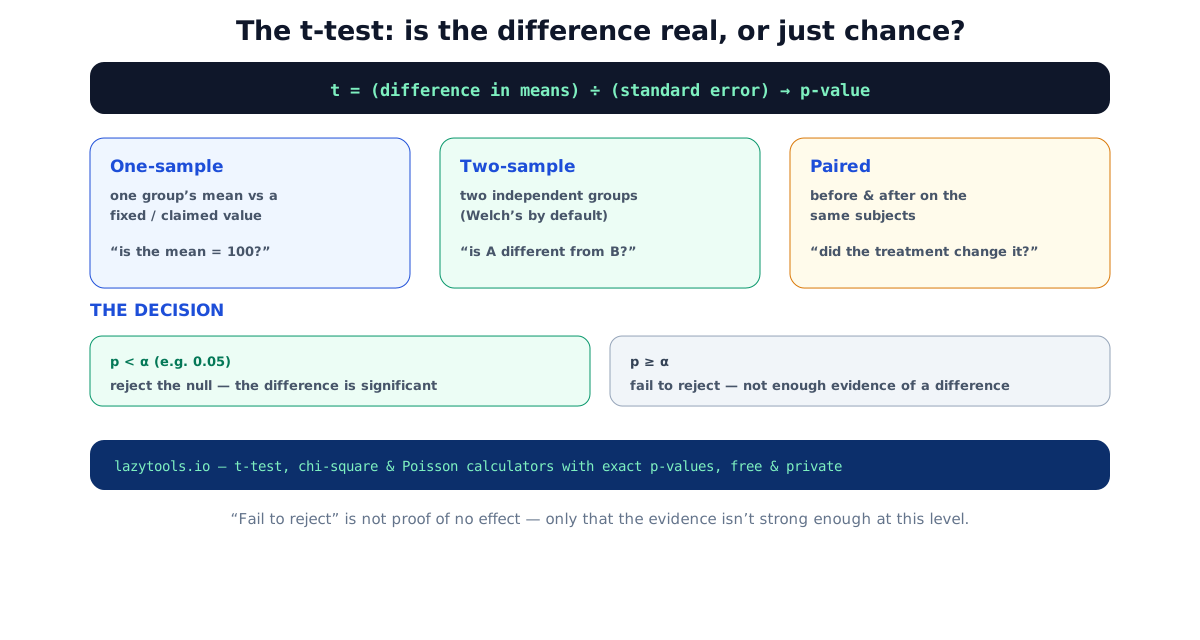
t = (difference in means) / (standard error of that difference)

The numerator is the effect you’re interested in; the denominator is how much the means would wobble from sampling alone. A big t means the difference is large relative to the noise. You then convert t (with its degrees of freedom) into a p-value using the t-distribution, the probability of a t this extreme if there were no real difference.

Why a t-distribution and not the normal curve? Because you rarely know the true spread of the population. You estimate it from your sample. That estimate is itself uncertain, so the t-distribution has slightly heavier tails than the standard normal, which widens your interval to account for that extra uncertainty. As the sample grows, the estimate sharpens and the t-distribution converges on the normal; by roughly 30 observations the two are almost indistinguishable.

Which t-test? Match it to your design

• One-sample. You have one group and a fixed reference value. “Is the mean fill weight really 500 g?” You test the sample mean against 500.
• Two-sample (independent), two separate groups. “Do method A and method B differ?” You compare the two group means. This is the most common case.
• Paired, two measurements on the same subjects. “Did blood pressure change after the drug?” You don’t compare group averages; you compute each person’s difference and test whether those differences average to zero. Pairing removes person-to-person variation, making it far more powerful than treating before and after as independent groups.

Getting this choice right matters more than any other decision, a paired design analysed as two independent samples throws away its biggest advantage.

Test	What you compare	Degrees of freedom	Typical question
One-sample	Sample mean vs a fixed value	n − 1	”Is the mean bottle fill really 500 g?”
Two-sample, pooled	Two group means (equal variance assumed)	n₁ + n₂ − 2	”Do methods A and B differ, similar spreads?”
Two-sample, Welch	Two group means (unequal variance allowed)	Welch, Satterthwaite (approx.)	”Do methods A and B differ, any spreads?”
Paired	Mean of within-subject differences vs 0	n − 1 (n = pairs)	“Did blood pressure change after the drug?”

The degrees of freedom (df) set which t-distribution you read the p-value from. Fewer df means heavier tails and a higher bar for significance, one more reason small samples struggle to reach it.

Welch or pooled?

For the two-sample test there are two flavours:

• Pooled (Student’s) assumes both groups have the same variance.
• Welch’s does not. It allows unequal variances and adjusts the degrees of freedom.

Default to Welch’s. It’s more reliable when the groups have different sizes or spreads, and it costs almost nothing when they’re similar. The old habit of running an equal-variance test is rarely worth it; reach for pooled only when equal variances are genuinely justified. A common older workflow, run an F-test for equal variance first, then pick pooled or Welch, is now discouraged, because that two-step “test-then-decide” procedure distorts the error rate. Just start with Welch’s.

A worked paired example

Suppose six patients have their systolic blood pressure measured before and after a drug, and the reductions (before − after, in mmHg) come out as: 8, 12, 5, 10, 6, 7.

1. Mean difference: (8 + 12 + 5 + 10 + 6 + 7) ÷ 6 = 48 ÷ 6 = 8 mmHg.
2. Standard deviation of the differences: the deviations from 8 are 0, 4, −3, 2, −2, −1; their squares sum to 34; dividing by n − 1 = 5 gives a variance of 6.8, so s ≈ 2.61 mmHg.
3. Standard error: s ÷ √n = 2.61 ÷ √6 ≈ 1.07 mmHg.
4. t statistic: 8 ÷ 1.07 ≈ 7.5, with df = n − 1 = 5.

A two-tailed test at df = 5 needs |t| ≈ 2.57 to clear α = 0.05. Our t of 7.5 is far past that, giving p < 0.001, strong evidence the drug lowered blood pressure. Note what pairing bought us: had we treated “before” and “after” as two independent groups of six, the large person-to-person variation in baseline pressure would have swamped the signal and the same data could easily have come out non-significant.

Reading the result, and the big trap

Compare the p-value to your significance level α (conventionally 0.05):

• p < α → reject the null hypothesis. The difference is “statistically significant”, unlikely to be chance.
• p ≥ α → fail to reject the null.

Here’s the mistake nearly everyone makes: failing to reject is not proof there’s no difference. It means you didn’t find enough evidence, which can happen simply because the sample was too small to detect a real effect (low statistical power). “Not significant” and “no effect” are different claims. And significance isn’t importance: with a huge sample, a trivially small difference can be statistically significant yet practically meaningless, so always look at the size of the difference too.

Report effect size, not just p

The p-value tells you whether an effect is detectable; it says nothing about how big it is. Pair it with two things:

• The raw difference and its confidence interval. “The drug lowered systolic pressure by 8 mmHg (95% CI 5.3 to 10.7)” is far more useful than “p < 0.001,” because it puts the effect in the units a reader actually cares about.
• A standardized effect size (Cohen’s d), the difference in means divided by a standard deviation, when you need to compare across studies that use different scales. As a rough convention Cohen suggested d ≈ 0.2 is small, 0.5 medium, and 0.8 large, though these are guidelines, not laws, and sensible thresholds vary by field.

Check the assumptions

A t-test is only as trustworthy as the conditions behind it:

• Approximate normality. The test assumes the data (or, for two samples, each group; for paired, the differences) are roughly normal. It’s fairly robust to mild departures, and with larger samples the central limit theorem carries the mean toward normality regardless. Heavy skew or strong outliers in a small sample are the real danger, inspect a histogram first.
• Independence. Observations should be independent of one another. Repeated measures on the same subject are not independent, which is exactly why the paired design exists.
• Equal variances, only for the pooled test. Welch’s version drops this requirement, which is why it’s the safer default.

When normality is badly violated and the sample is small, a rank-based alternative, the Mann, Whitney U test for two independent groups, or the Wilcoxon signed-rank test for paired data, is often the better choice.

Run it

The t-test calculator does all three types from summary statistics (means, standard deviations and sample sizes), defaults to Welch’s for two samples, handles one- or two-tailed hypotheses, and gives the exact t, degrees of freedom, p-value and a plain-English significance verdict. For categorical counts instead of means, use the chi-square test; to turn a test statistic you already have into a p-value, use the p-value calculator. Everything runs in your browser, your data is never uploaded.

---

The t-test assumes roughly normal data (or a large enough sample for the central limit theorem to apply) and, for the pooled version, equal variances. p-values come from the exact Student t-distribution. This is educational content; for high-stakes analysis, check the assumptions and consider effect size and power. Source: standard mathematical-statistics treatment of the t-test (e.g. Student 1908; Welch 1947).